SITCOMTN-163

Source Selection for Abell 360 in LSSTComCam Data Preview 1#

Abstract

We cover the source selection done for the Abell 360 LSSTComCam cluster study focusing on color and photo-z cuts. Identification of cluster members via the red sequence and photo-z offers a science focused validation of photometry with LSSTComCam. We are able to cross-match with DESI spectroscopic redshifts to offer an independent validation suite on photo-z estimates. We make various color and photo-z cuts to generate N(z)s and shear profiles. We find that both cuts are quite robust to various choices made and can produce a shear profile for Abell 360. Both methods should be applicable to generating a consistent mass estimate for the cluster.

DOI: https://doi.org/10.71929/rubin/2571157

Introduction#

The Rubin LSSTComCam [Stalder et al., 2022, Stalder et al., 2020, SLAC National Accelerator Laboratory and NSF-DOE Vera C. Rubin Observatory, 2024] observing campaign undertaken at the end-of-year 2024 covered seven fields, among which include the low ecliptic latitude Rubin SV 38 7 field containing the Abell 360 (A360) galaxy cluster. A360 is an intermediate mass cluster ($M_{500,c} = 4.3\times 10^14 M_\odot$[Hilton et al., 2021] at z=0.22 [Quintana and Ramirez, 1995] that we use as a commissioning demonstrator of Rubin capabilities for cluster weak lensing (WL) studies. In order to best measure the shear profile of the cluster, we would ideally only measure the shapes of galaxies that are lensed by the cluster, i.e. source galaxies that are behind the cluster. This can be done by identifying and removing cluster members via the red sequence, an overdensity on a color-magnitude diagram caused by the cluster members, or by removing objects near and below the redshift of the cluster.

We will discuss both methods, associated verification, the estimated redshift distribution, $N(z)$, from each method, and the shear profile from the various sources.

This technote is one part of a series studying A360 in order to both stress test the commissioning camera and demonstrate the technical capabilities of the Vera Rubin Observatory. We study the quality of the PSF modeling and impact it can have on cluster WL in [Combet et al., 2025], implementation of cell-based coadds and subsequent use for Metadetect [Sheldon et al., 2023] in [Gorsuch, 2025], photometric calibration in insert here, use of Anacal [Li et al., 2023] to produce a shear profile in [Li, 2025], and background subtraction in this field and Fornax in insert here.

Dataset#

The Rubin SV 38 7 field has been observed in g (44 visits), r (55 visits), i (57 visits) and z (27 visits) [Guy et al., 2025] with no visits in u and y-band. The Data Preview 1 (DP1) Object catalog [NSF-DOE Vera C Rubin Observatory, 2025, NSF-DOE Vera C. Rubin Observatory, 2025]includes various flux measurements including cModel [Abazajian et al., 2004] and GaaP [Kuijken, 2008] along with HSM shape measurements [Mandelbaum et al., 2006, Hirata and Seljak, 2003]. The second moments of the light profile of objects, $Q_{ij}$, and of the PSF at each object, $Q^{\textrm{PSF}}_{ij}$, are included which can be combined to create size estimate $T = Q_{xx} + Q_{yy}$ of the object and PSF at that point. These are in turn used to calculate the HSM resolution factor [Mandelbaum et al., 2018],$R = 1-\frac{T_\textrm{PSF}}{T_\textrm{I}}$, which compares the resolution of a galaxy to the PSF in order to remove stars and poor quality objects Photometric redshift estimates are not included in the DP1 catalog but have been created as outlined in [Graham, 2025].

The DP1 catalog is divided into large tracts which is subdivided into patches. We first gather all data in nearby tracts and then apply basic quality flags to remove objects that have caused a failure in the flux measurements, namely from saturation, cosmic rays, and spurious detections. Each quality flag is a boolean which is set to True if the algorithm fails to run on that object for whatever reason. The flags and number of objects affected by the flag are listed in Table 1.

Table 1 Quality flags and number of objects affected by flag.#
Flag Name	Number of Objects
refExtendedness	24892
i_iPSF_flag	62462
i_hsmShapeRegauss_flag	91836
g_cModel_flag	4016
r_cModel_flag	4228
i_cModel_flag	4137
z_cModel_flag	3173
g_gaapFlux_flag	0
r_gaapFlux_flag	0
i_gaapFlux_flag	6
z_gaapFlux_flag	0

Within 0.5 degrees of the brightest central galaxy (BCG) located at (RA, DEC) = $(37.865017^{\circ}, 6.982205^{\circ})$ we have 58676 objects with measurements in griz bands. Star-galaxy separation is done using the refExtendedness flag which will flag objects if $\frac{\textrm{flux}_\textrm{psf}}{\textrm{flux}_\textrm{cModel}} < .985$ [Bosch et al., 2018] as galaxies giving 52309 galaxies (89%) and 6367 stars (11%). The counts per bin of galaxies only is shown in Fig. 1 with griz bands reaching an estimated depth of 24.9, 24.5, 24.3, and 23.6 mags respectively. The depths are estimated by using the peak of the galaxy magnitude distribution below. These limits are not derived from synthetic source injection and should be treated as rough guides to the true limits.

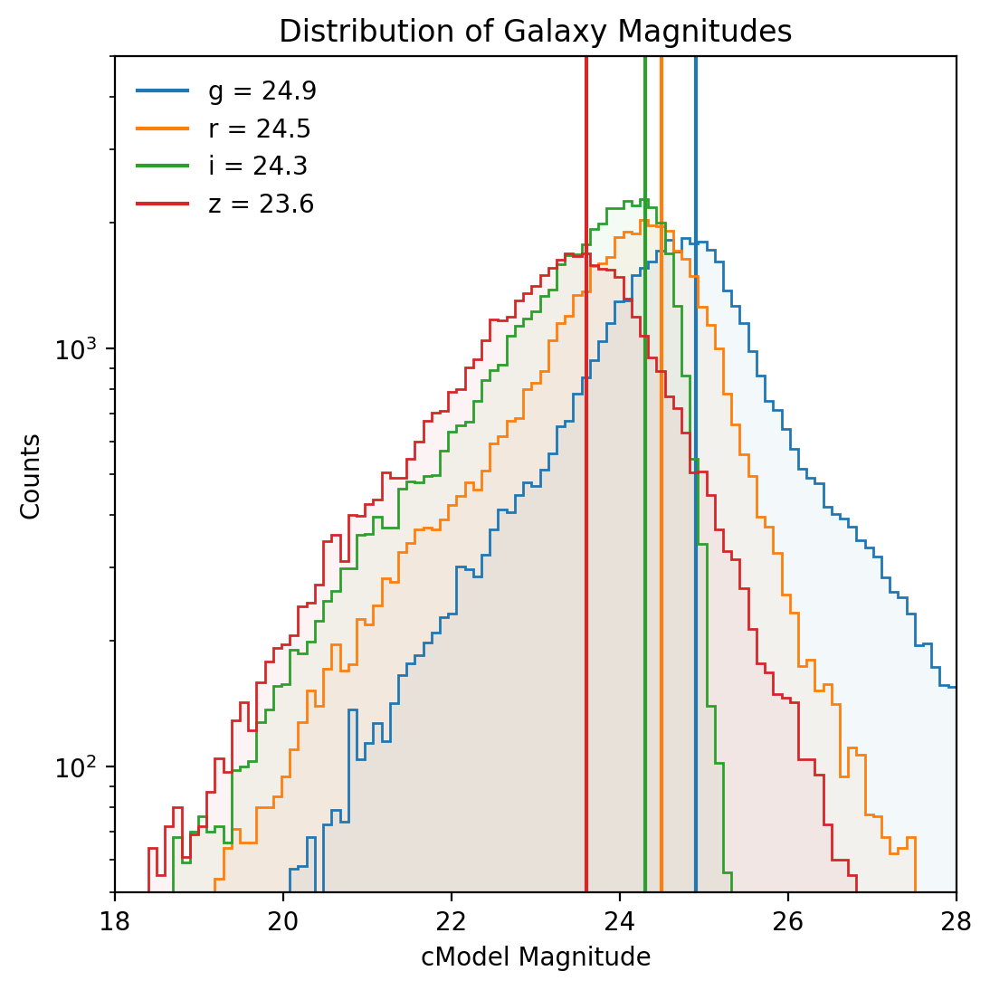
_images/galaxy_dist.png — Fig. 1 Distribution of galaxy magnitudes with (approximate) limiting magnitude shown as histogram with *griz* corresponding to blue, orange, green, and red and the magnitude limit per band shown as solid vertical line in the same color.#

Color-cuts#

We can select cluster members by identifying the red sequence galaxies in a color-magnitude diagram. Due to fewer observations in z we focus on the gri bands and the colors (g-r, r-i, g-i) from this set. We use cModel fluxes for magnitudes and GaaP1p0 fluxes for colors.

To identify the red sequence we first restrict to detections within 0.1 degrees (1.3 Mpc) of the BCG which leaves 2194 galaxies. The color-magnitude diagram is shown below in Fig. 2

_images/CMD_nors.png — Fig. 2 Color-magnitude diagrams for galaxies near the BCG using cModel r magnitude on x-axis and GaaP calculated colors on the y-axis. From left to right we show the *g-i*, *r-i*, and *g-r* colors with the red sequence overdensity clearly visible.#

The red sequence is identified per color by eye with a limiting magnitude of $r < 24$ applied and shown in Fig. 3 giving 286, 316, 286 objects in the g-i, r-i, and g-r CMDs respectively. Requiring that an object be in all three red sequences restricts us to 216 objects and is shown in Fig. 4.

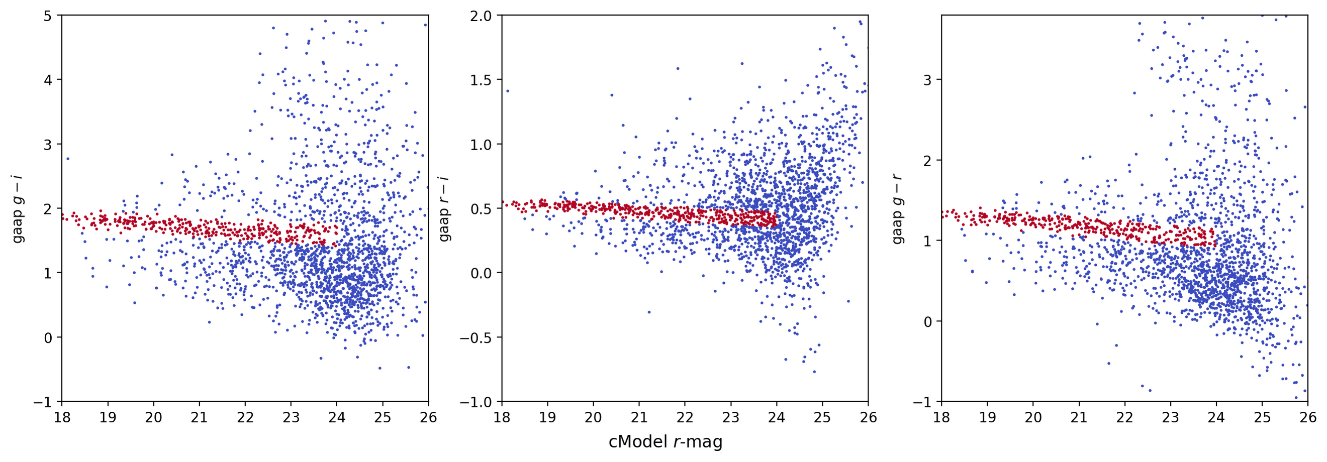
_images/CMD_rs.png — Fig. 3 Red sequence members identified by eye and adding a magnitude limit of $r < 24$. From left to right we show the *g-i*, *r-i*, and *g-r* colors.#

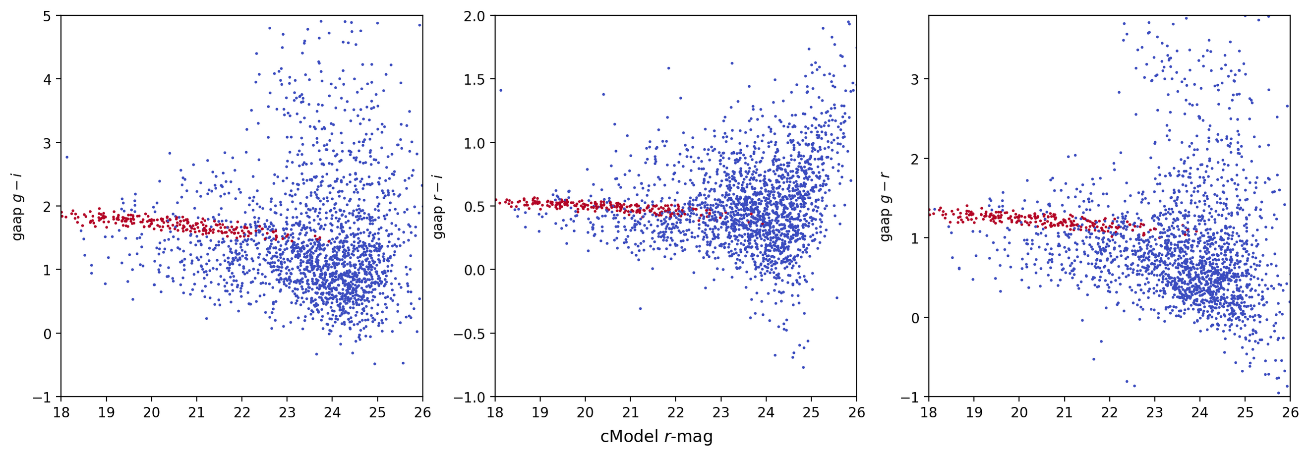
_images/CMD_all_rs.png — Fig. 4 Multi-color red sequence members. From left to right we show the *g-i*, *r-i*, and *g-r* colors.#

When applying the color cuts to the sample (within 0.5$^\circ$ of the BCG), we remove 873 galaxies and remain with 57803 galaxies.

Photo-Z Selection#

Photometric redshift (photo-z) selection is another option to remove any objects that would not be lensed by the cluster and thus dilute the signal. Photo-zs were estimated using FlexZBoost (FZBoost) [Dalmasso et al., 2020, Izbicki et al., 2017], TreePhotoZ (TPZ) [Carrasco Kind and Brunner, 2013], k-Nearest Neighbors (kNN) [Schmidt et al., 2023], and Bayesian Photo-zs (BPZ) [Benitez, 2000] as implemented in RAIL [Schmidt et al., 2023] using the 4 available bands griz on cModel fluxes. These estimators were chosen as kNN and BPZ will be provided by the Rubin project for future data releases while we expect FZB and TPZ to be readily available from the community. The estimators were trained on the same 4 bands in the Extended Chandra Deep Field South (ECDFS) field and then applied to the cluster field. We apply the same cuts as in Table 1 and also require that width of the photo-$z$ estimate, $\sigma_z$, be small ($\sigma_z < 0.25$) for each object. Along with removing spurious and extremely faint objects, we remove objects that are likely causing large issues for photo-z estimators due to the missing u and y band. The redshift distribution, $N(z)$, after applying these quality cuts is shown in Fig. 5 along with the location of our subsequent photo-z cut to remove cluster members. That cut is placed at $z = 0.37 = 0.22 + .15$ where the additional $0.15$ acts as a buffer to help lower dilution from the cluster and is placed on mean photo-z estimate for all techniques except kNN for which we use median due to implementation issues.

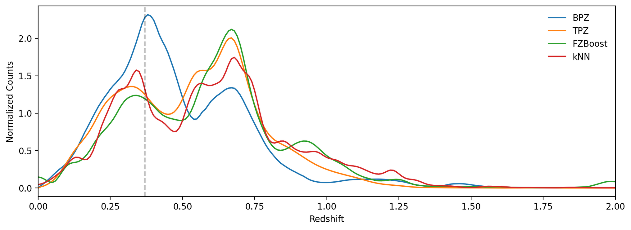
_images/quality_cuts_nz.png — Fig. 5 Photometric redshift distribution for the galaxy sample (within 0.5 deg, or 6.4 Mpc, of the central BCG and with 20 < i < 24) for 4 photometric redshift estimators. BPZ is shown in blue, TPZ in orange, FZBoost in green, and kNN in red. A faint dashed line is included where the cluster cut will be placed ($z = 0.37$).#

In this field, we have overlap with the DESI [Collaboration et al., 2025] BGS [Hahn et al., 2023], ELG [Raichoor et al., 2023], and LRG [Zhou et al., 2023] catalogs, shown in Fig. 6, which allows us to perform simple external validation on the four redshift techniques. After matching we have 2728 galaxies with spectroscopic redshifts. Details on the matching and breakdown can be found in [Graham, 2025].

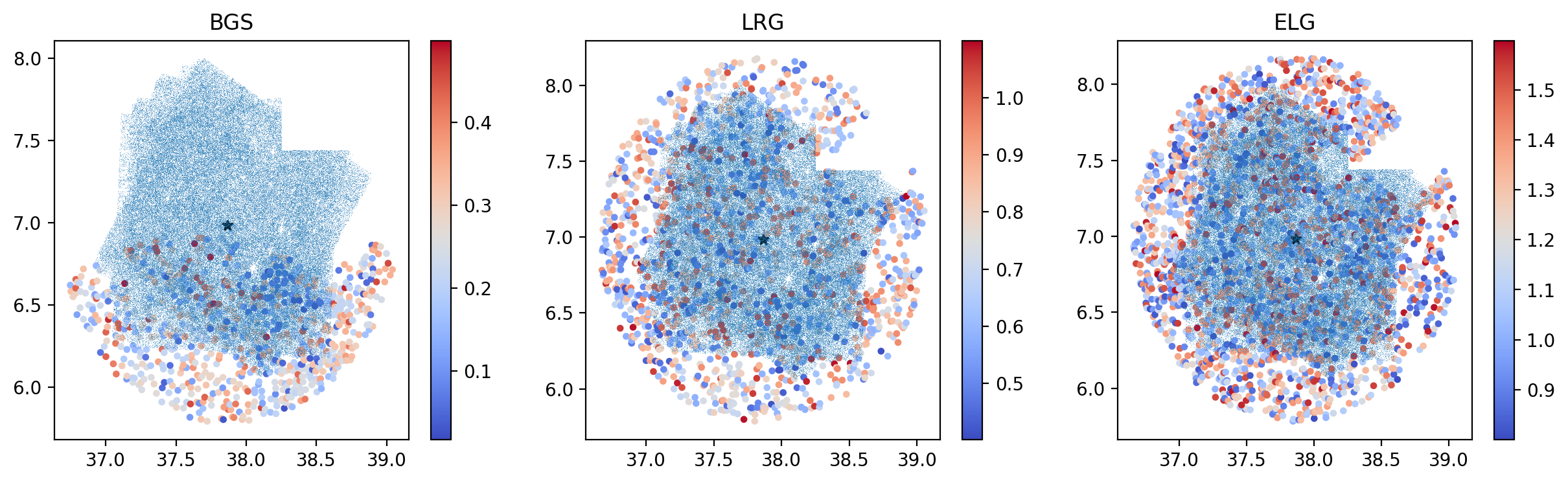
_images/desi_location.png — Fig. 6 Overlap between SV 38-7 field and various DESI subsamples. Note that the BGS sample that covers the low-z regime does not uniformly cover the region and thus we are incomplete in this space. From [Graham, 2025].#

To validate the techniques, we compare the photo-z for objects with matches to the DESI sample which we show in Fig. 7 without placing a cut on $\sigma_z$ and in Fig. 8 to highlight the improvement in photo-z estimate when using this cut. Even without placing the cut, most techniques perform quite well up to $z < 0.8$ but then suffer onwards. It is likely that this is caused by a mismatch between the training sample and validation sample (ELGs) which can cause systematic issues. Once a cut on $\sigma_z$ is placed (Fig. 8), we have much higher quality photo-z estimates that are able to predict to higher redshifts quite well.

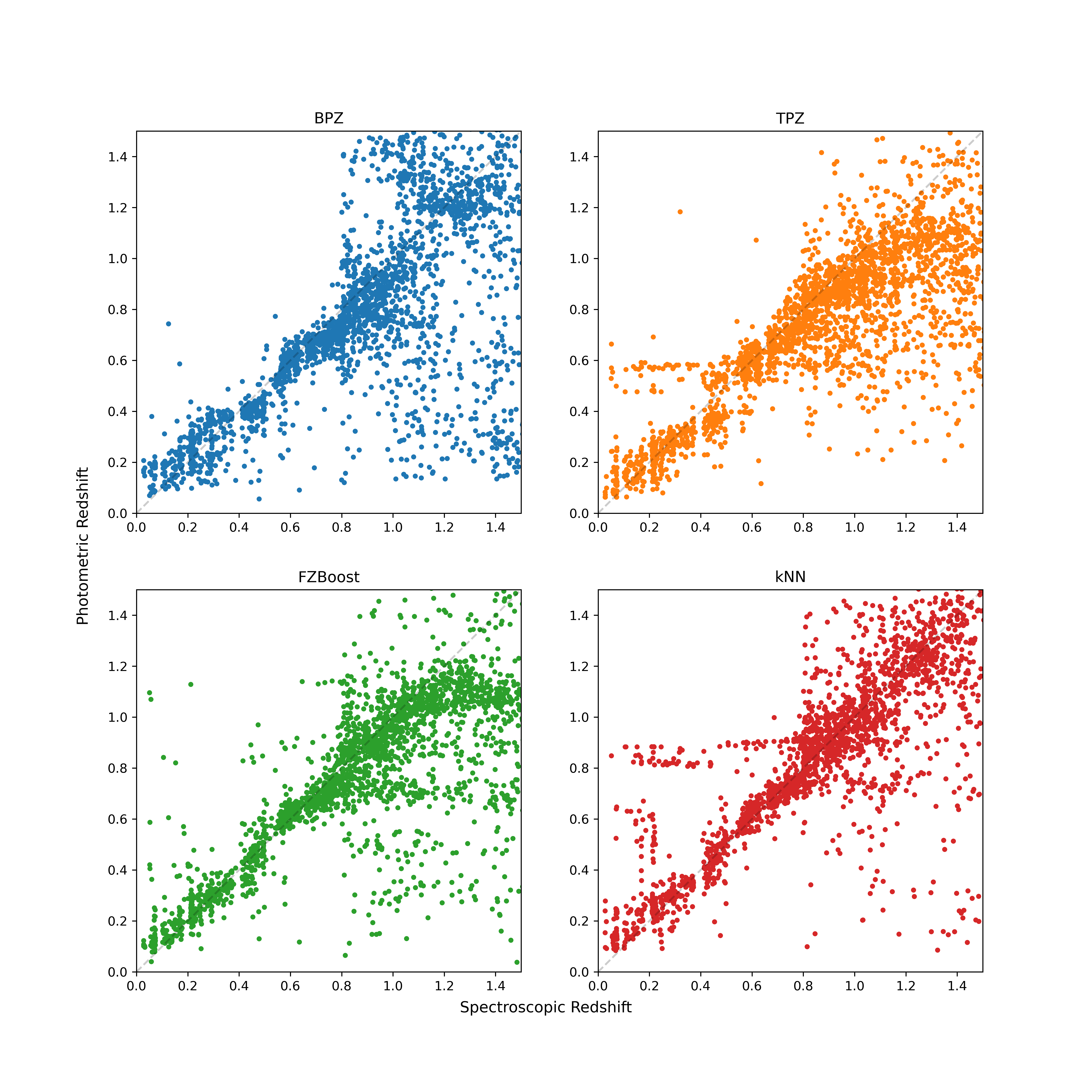
_images/scatter_compare_nocut.png — Fig. 7 Photometric redshift estimates versus matched spectroscopic redshifts from DESI for the four methods studied in this technote with minimal quality cuts applied (Table 1 only), namely no $\sigma_z$ cut applied on the photometric redshift estimates. In the upper left in blue we display BPZ, upper right in orange TPZ, lower left in green FZBoost, and lower right in red kNN. The issues at high redshift ($z >0.8$) may be caused by mismatch between the training and validation sets.#

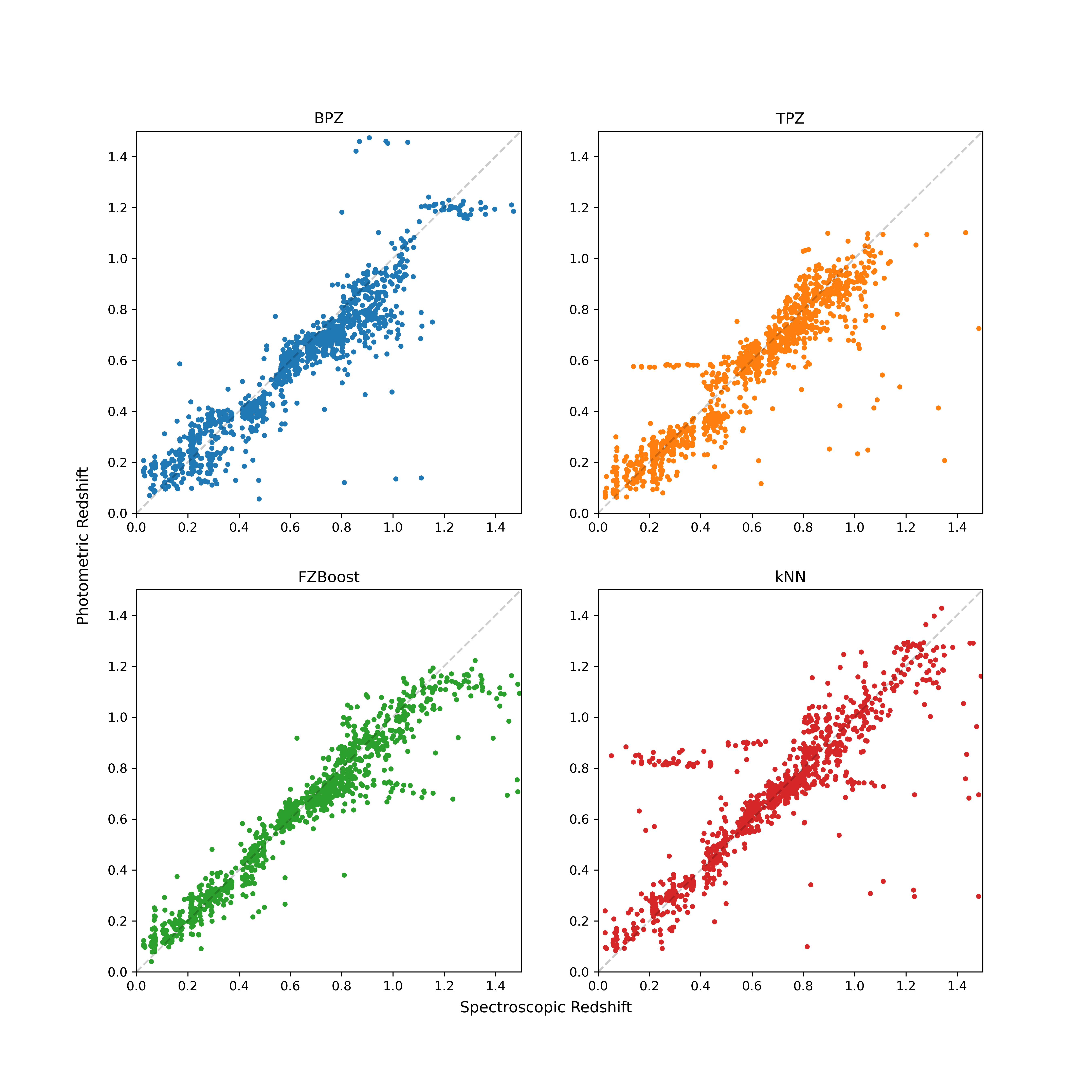
_images/scatter_compare_cut.png — Fig. 8 Photometric redshift estimates versus matched spectroscopic redshifts from DESI for the four methods studied in this technote with quality cuts applied (Table 1) along with requiring $\sigma_z < 0.25$. In the upper left in blue we display BPZ, upper right in orange TPZ, lower left in green FZBoost, and lower right in red kNN. Note the improvement from Fig. 7.#

For more details on the matching and performance of other photo-z estimators on this field, and DP1 in general, please refer to [Graham, 2025].

Red Sequence Redshift#

Checking the redshift of the red sequence members acts as a self-consistency check for photometry and photo-z estimates. Applying the same red sequence cuts seen in Fig. 3 on the DESI matched sample we can directly read off spectroscopic redshifts which we show in Fig. 9. We can further validate the photo-z estimators by comparing the DESI N(z) for the red sequence to the photometric N(z) which we display in Fig. 10.

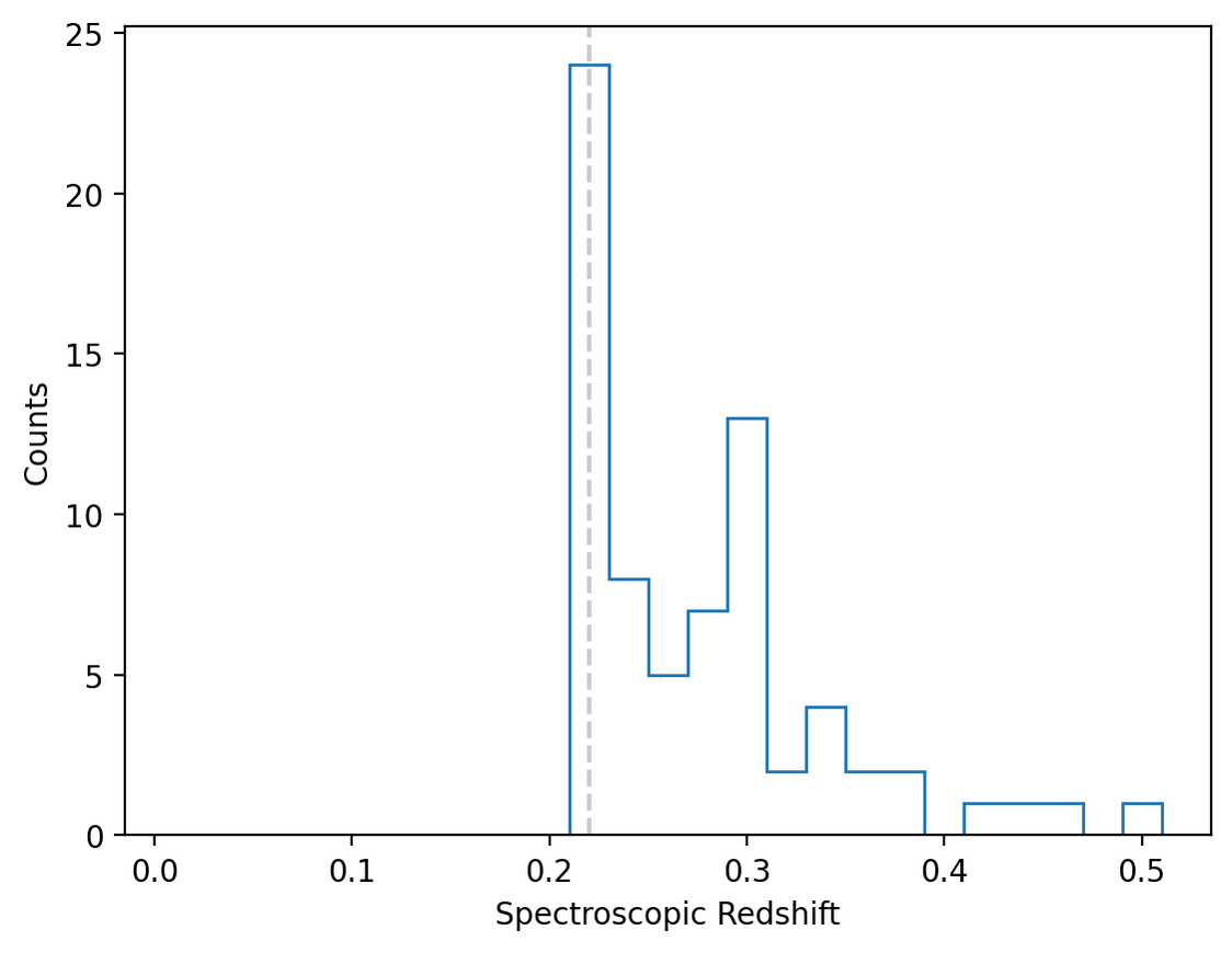
_images/matched_redseq_z.png — Fig. 9 Histogram of spectroscopic redshifts from DESI matched red sequence galaxies in blue. The cluster location is shown as a faint dashed gray line at $z=0.22$.#

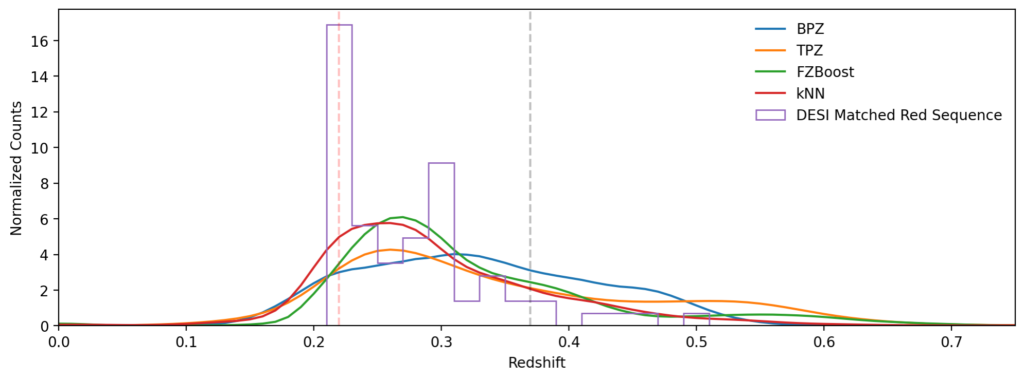
_images/matched_redseq_z-pzpdf.png — Fig. 10 Histogram of spectroscopic redshifts from DESI matched red sequence galaxies in purple along with the N(z) from the photo-z estimators. The cluster location is shown as a faint dashed red line at $z=0.22$ and a solid gray line at $z=0.37$ for the cut applied on the photo-z sample.#

The peak of the DESI distribution gives us confidence that we are removing cluster members but the tail is slightly concerning. The color-cuts could be optimized to reduce the size of the tail, but due to the limited coverage in the area from the DESI low-z catalogs and varying selection functions between the two instruments, we only use it as validation.

Shear profiles and N(z)#

With a variety of source selection methods available, we can compare the $N(z)$ and final HSM shear profile from each source to see if the subsamples are relatively stable. Following [Li et al., 2022], we also apply a set of weak lensing cuts to both samples to ensure that the sample has good quality shape measurements. The cuts and values used are listed below in Table 2

Table 2 Weak Lensing Cuts#
Column
refExtendedness > 0.5
20 $\leq$ i_cModel_mag $\leq$ 24
$\frac{\textrm{i_cModelFlux}}{\textrm{i_cModelFluxErr}} \geq 10$
i_hsmShapeRegauss_e1$^2$ + i_hsmShapeRegauss_e2$^2 \leq 4$
$1-\frac{T_\textrm{PSF}}{T_\textrm{I}} \geq 0.3$
i_blendedness $\leq 0.42$

Shear Profile#

To calculate the shear profile for each subsample when applying color cuts or photo-z cuts, we first convert from $e_1$ and $e_2$ to $\gamma_1$ and $\gamma_2$ by applying HSC Y1 shear calibration [Mandelbaum et al., 2018, Mandelbaum et al., 2018].

Once calibrated, we can convert the shears to tangential and cross components using the cluster BCG, located at (RA, DEC) = (37.865017, 6.982205), using

\[\begin{split}\gamma_+ &= -\gamma_1 \cos{2\phi} - \gamma_2\sin{2\phi} \\ \gamma_\times &= \gamma_1 \sin{2\phi} - \gamma_2\cos{2\phi}\end{split}\]

Once calibrated and converted, we can extract a shear profile centered on the BCG and vary the color cuts applied which we present in Fig. 11. Notably, the profile is quite insensitive to the specific color cut chosen with the tangential components located at similar values and the cross component mostly consistent with 0. Similarly, we can apply our photo-$z > 0.37$ cut on BPZ, TPZ, FZBoost, and kNN to produce a source sample that we calculate the shear profile of in Fig. 12. While there is a larger spread on the value of the $\gamma_+$ between the cuts, the signal is quite similar to the color-cut profile and similarly passes the null test of $\gamma_\times = 0$ aside from the fourth bin which is high in the color-cut profile as well.

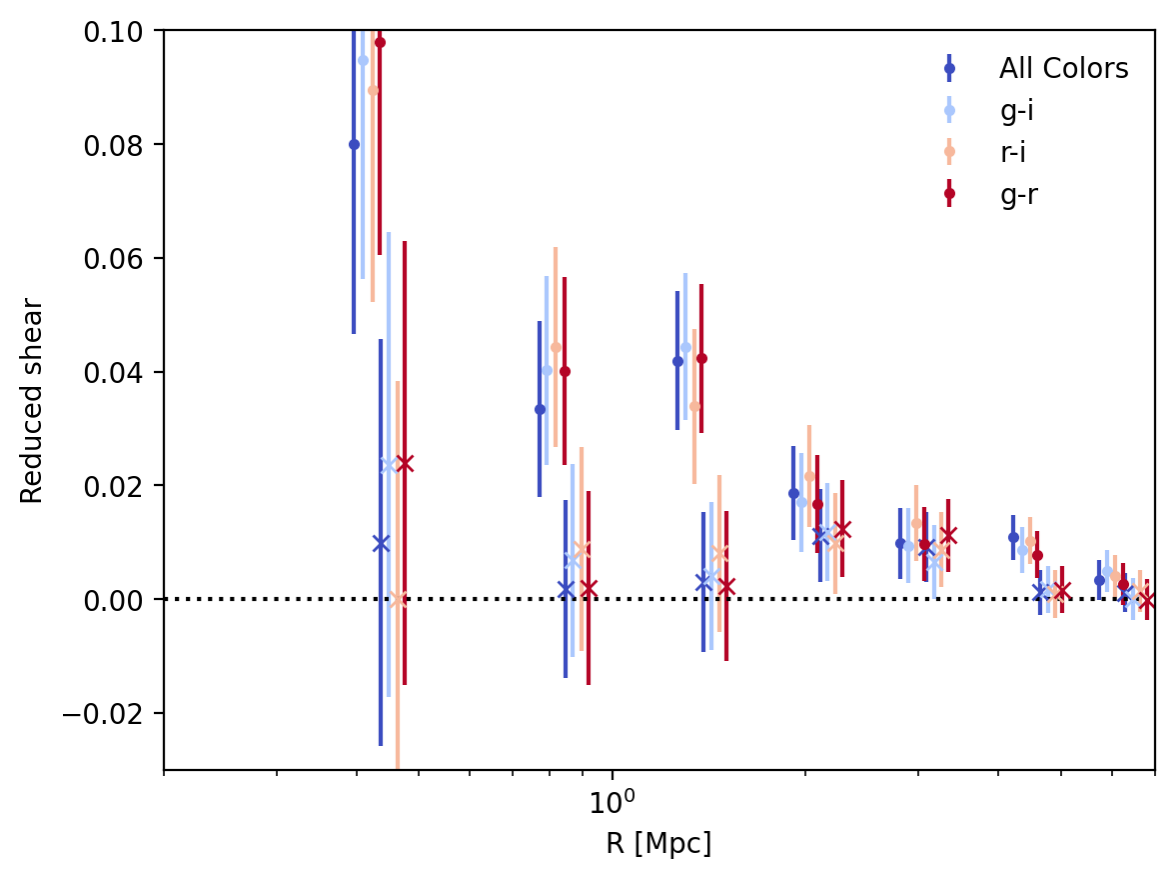
Fig. 11 The shear profile with varying color cuts. The tangential shear component is shown with circular points and cross shear component with x points. The error bar represents a 95% confidence interval from bootstrapped samples. “All colors” refers to using all three red sequences and is shown in dark blue, “g-i” uses points found only on the $g-i$ red sequence and is shown in light blue, “r-i” for the $r-i$ redsequence and shown in light red, and “g-r” for the $g-r$ redsequence and shown in dark red. The points are staggered on the x-axis for clarity.#

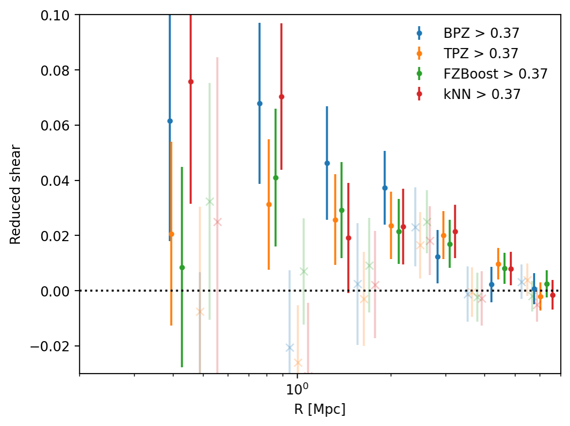
Fig. 12 The shear profile with varying photo-z estimators all cut at $z=0.37$. BPZ is shown in blue, TPZ in orange, FZBoost in green, and kNN in red. The cross shear term is shown in the same colors but much fainter and with a “x” at the point instaed of a dot. The data is staggered on the x-axis for clarity.#

N(z)#

To estimate the mass of a cluster, we need the $N(z)$ of our lensing sample which we present here. Ideally, the two methods (color-cuts and photo-z cut) would produce similar $N(z)$s. To estimate the $N(z)$ when using color cuts, we use the ECDFS photo-zs and apply the same red sequence and weak lensing cuts. The ECDFS field was observed in 6 bands which enables higher quality photo-z estimates and by using the same instrument, we have a very similar selection function between the two fields. To offset the difference in depth between the two fields we restrict to $i < 23.5$ and SNR$_i \geq 10$. The increased brightness limit was chosen to keep the magnitude limit as the dominant cut in the sample (versus the SNR cut) which is not the case at $i = 24$ for the cluster field. The $N(z)$ with the color cut transferred is presented in Fig. 13 and the $N(z)$ directly in the field in Fig. 14.

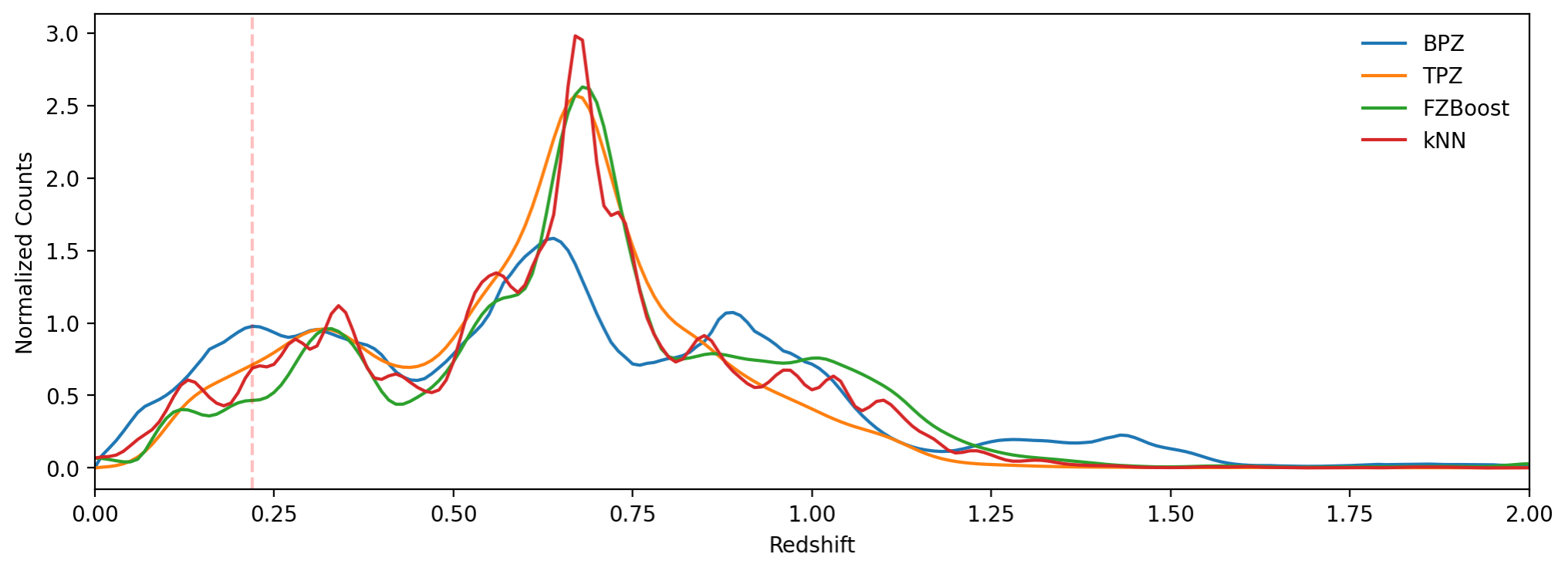
_images/ECDFS_nz.png — Fig. 13 $N(z)$ from 6 band photo-z estimates when applying quality cuts, weak lensing cuts, and color cuts all transferred to the ECDFS sample. BPZ is shown in blue, TPZ in orange, FZboost in green, and kNN in red. A dashed red line is added to show the location of the cluster.#

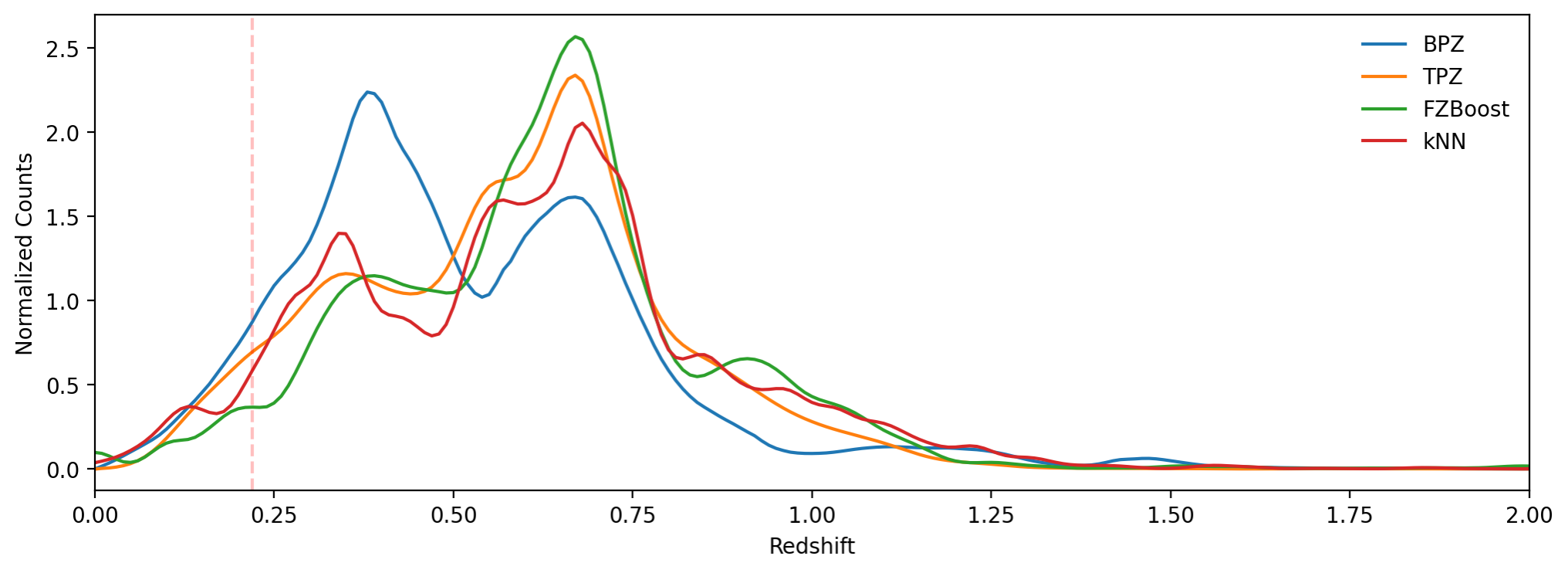
_images/cc_cuts_4bandsnz.png — Fig. 14 $N(z)$ from 4 band photo-z estimates when applying quality cuts, weak lensing cuts, and color cuts. BPZ is shown in blue, TPZ in orange, FZboost in green, and kNN in red. A dashed red line is added to show the location of the cluster.#

On the photo-z cut, we remove objects that have their central statistic (mean) below $z=0.37$ but the $N(z)$ will still have support in that range from objects near the cut with wide distributions. The distribution is plotted in Fig. 15.

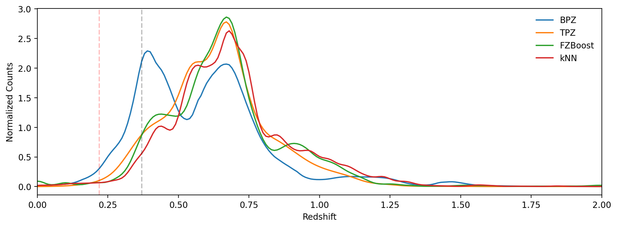
_images/wl_cuts_nz.png — Fig. 15 $N(z)$ from the 4 photo-z techniques after applying quality cuts, a $\sigma_z$ cut, weak lensing cuts, and $z \leq 0.37$ cut. BPZ is shown in blue, TPZ in orange, FZBoost in green, and kNN in red. A dashed red line is added to show the location of the cluster and a dashed gray line is added to show the location of the photo-z cut.#

All 3 $N(z)$ distributions peak at $z\approx 0.6$ and approach zero by $z\approx 1.3$. Both of the 4-band distributions, Fig. 14 and Fig. 15, show a peak for BPZ near 0.4 which is concerning. The photo-z $N(z)$ is very good at removing low redshift objects as seen by the flat distribution between the red and gray lines in Fig. 14.

Conclusion#

In this technote we have outlined the source selection for studying A360 in order to enable cluster weak lensing and verify the science pipelines. We find that the high quality photometry makes the red sequence easily identifiable and the source selection fairly consistent between the multiple colors. When using photometric redshifts, we are able to recreate a similar signal and validate against the DESI spectroscopic redshifts which acts as a completely external test suite for photometric redshifts which were not trained on DESI spec-zs. In total, the two methods give confidence that the combination of object detection and deblending, galaxy photometry, and photometric redshift estimates from the Vera Rubin observatory will enable high quality cluster science in the years to come.

References#

[1]

Narciso Benitez. Bayesian photometric redshift estimation. The Astrophysical Journal, 536(2):571–583, June 2000. URL: http://dx.doi.org/10.1086/308947, doi:10.1086/308947.

[2]

DESI Collaboration, M. Abdul-Karim, A. G. Adame, D. Aguado, J. Aguilar, S. Ahlen, S. Alam, G. Aldering, D. M. Alexander, R. Alfarsy, L. Allen, C. Allende Prieto, O. Alves, A. Anand, U. Andrade, E. Armengaud, S. Avila, A. Aviles, H. Awan, S. Bailey, A. Baleato Lizancos, O. Ballester, A. Bault, J. Bautista, S. BenZvi, L. Beraldo e Silva, J. R. Bermejo-Climent, F. Beutler, D. Bianchi, C. Blake, R. Blum, A. S. Bolton, M. Bonici, S. Brieden, A. Brodzeller, D. Brooks, E. Buckley-Geer, E. Burtin, R. Canning, A. Carnero Rosell, A. Carr, P. Carrilho, L. Casas, F. J. Castander, R. Cereskaite, J. L. Cervantes-Cota, E. Chaussidon, J. Chaves-Montero, S. Chen, X. Chen, T. Claybaugh, S. Cole, A. P. Cooper, M. -C. Cousinou, A. Cuceu, T. M. Davis, K. S. Dawson, R. de Belsunce, R. de la Cruz, A. de la Macorra, A. de Mattia, N. Deiosso, J. Della Costa, R. Demina, U. Demirbozan, J. DeRose, A. Dey, B. Dey, J. Ding, Z. Ding, P. Doel, K. Douglass, M. Dowicz, H. Ebina, J. Edelstein, D. J. Eisenstein, W. Elbers, N. Emas, S. Escoffier, P. Fagrelius, X. Fan, K. Fanning, V. A. Fawcett, E. Fernández-García, S. Ferraro, N. Findlay, A. Font-Ribera, J. E. Forero-Romero, D. Forero-Sánchez, C. S. Frenk, B. T. Gänsicke, L. Galbany, J. García-Bellido, C. Garcia-Quintero, L. H. Garrison, E. Gaztañaga, H. Gil-Marín, O. Y. Gnedin, S. Gontcho A Gontcho, A. X. Gonzalez-Morales, V. Gonzalez-Perez, C. Gordon, O. Graur, D. Green, D. Gruen, R. Gsponer, C. Guandalin, G. Gutierrez, J. Guy, C. Hahn, J. J. Han, J. Han, S. He, H. K. Herrera-Alcantar, K. Honscheid, J. Hou, C. Howlett, D. Huterer, V. Iršič, M. Ishak, A. Jacques, J. Jimenez, Y. P. Jing, B. Joachimi, S. Joudaki, R. Joyce, E. Jullo, S. Juneau, N. G. Karaçaylı, T. Karim, R. Kehoe, S. Kent, A. Khederlarian, D. Kirkby, T. Kisner, F. -S. Kitaura, N. Kizhuprakkat, H. Kong, S. E. Koposov, A. Kremin, A. Krolewski, O. Lahav, Y. Lai, C. Lamman, T. -W. Lan, M. Landriau, D. Lang, J. U. Lange, J. Lasker, J. M. Le Goff, L. Le Guillou, A. Leauthaud, M. E. Levi, S. Li, T. S. Li, K. Lodha, M. Lokken, Y. Luo, C. Magneville, M. Manera, C. J. Manser, D. Margala, P. Martini, M. Maus, J. McCullough, P. McDonald, G. E. Medina, L. Medina-Varela, A. Meisner, J. Mena-Fernández, A. Menegas, M. Mezcua, R. Miquel, P. Montero-Camacho, J. Moon, J. Moustakas, A. Muñoz-Gutiérrez, D. Muñoz-Santos, A. D. Myers, J. Myles, S. Nadathur, J. Najita, L. Napolitano, J. A. Newman, F. Nikakhtar, R. Nikutta, G. Niz, H. E. Noriega, N. Padmanabhan, E. Paillas, N. Palanque-Delabrouille, A. Palmese, J. Pan, Z. Pan, D. Parkinson, J. Peacock, W. J. Percival, A. Pérez-Fernández, I. Pérez-Ràfols, P. Peterson, J. Piat, M. M. Pieri, M. Pinon, C. Poppett, A. Porredon, F. Prada, R. Pucha, F. Qin, D. Rabinowitz, A. Raichoor, C. Ramírez-Pérez, S. Ramirez-Solano, M. Rashkovetskyi, C. Ravoux, A. H. Riley, A. Rocher, C. Rockosi, J. Rohlf, A. J. Ross, G. Rossi, R. Ruggeri, V. Ruhlmann-Kleider, C. G. Sabiu, K. Said, A. Saintonge, L. Samushia, E. Sanchez, N. Sanders, C. Saulder, E. F. Schlafly, D. Schlegel, D. Scholte, M. Schubnell, H. Seo, A. Shafieloo, R. Sharples, J. Silber, M. Siudek, A. Smith, D. Sprayberry, J. Suárez-Pérez, J. Swanson, T. Tan, G. Tarlé, P. Taylor, G. Thomas, R. Tojeiro, R. J. Turner, W. Turner, L. A. Ureña-López, R. Vaisakh, M. Valluri, M. Vargas-Magaña, L. Verde, M. Walther, B. Wang, M. S. Wang, W. Wang, B. A. Weaver, N. Weaverdyck, R. H. Wechsler, M. White, M. Wolfson, J. Yang, C. Yèche, S. Youles, J. Yu, S. Yuan, E. A. Zaborowski, P. Zarrouk, H. Zhang, C. Zhao, R. Zhao, Z. Zheng, R. Zhou, H. Zou, S. Zou, and Y. Zu. Data release 1 of the dark energy spectroscopic instrument. 2025. URL: https://arxiv.org/abs/2503.14745, arXiv:2503.14745.

[3]

C. Combet, A. Plazas Malagón, S. Fu, P. Adari, I. Dell'Antonio, A. Englert, M. Gorsuch, K. Laliotis, P.-F. Léget, E. Pedersen, A. von der Linden, Y. Zhang, and et al. (TBC). PSF assessment in the field of Abell 360 and shapeHSM shear profile using LSSTComCam data. Commissioning Technical Note SITCOMTN-161, Vera C. Rubin Observatory, July 2025. URL: https://sitcomtn-161.lsst.io/.

[4]

N. Dalmasso, T. Pospisil, A.B. Lee, R. Izbicki, P.E. Freeman, and A.I. Malz. Conditional density estimation tools in python and r with applications to photometric redshifts and likelihood-free cosmological inference. Astronomy and Computing, 30:100362, January 2020. URL: http://dx.doi.org/10.1016/j.ascom.2019.100362, doi:10.1016/j.ascom.2019.100362.

[5]

Miranda R. Gorsuch. Testing the implementation of Metadetection and Cell-Based Coadds on Abell 360 ComCam data. Commissioning Technical Note SITCOMTN-162, Vera C. Rubin Observatory, July 2025. URL: https://sitcomtn-162.lsst.io/.

[6] (1,2,3,4)

Melissa Graham. Photometric redshifts for ComCam data. Commissioning Technical Note SITCOMTN-154, Vera C. Rubin Observatory, June 2025. URL: https://sitcomtn-154.lsst.io/.

[7]

Leanne P. Guy, Keith Bechtol, Eric Bellm, Bob Blum, Gregory P. Dubois-Felsmann, Melissa L. Graham, Željko Ivezić, Robert H. Lupton, Phil Marshall, Colin T. Slater, and Michael Strauss. Rubin Observatory Plans for an Early Science Program. Technical Note RTN-011, Vera C. Rubin Observatory, May 2025. URL: https://rtn-011.lsst.io/, doi:10.5281/zenodo.5683848.

[8]

Rafael Izbicki, Ann B. Lee, and Peter E. Freeman. Photo-$z$ estimation: An example of nonparametric conditional density estimation under selection bias. The Annals of Applied Statistics, 11(2):698 – 724, 2017. URL: https://doi.org/10.1214/16-AOAS1013, doi:10.1214/16-AOAS1013.

[9]

K. Kuijken. Gaap: psf- and aperture-matched photometry using shapelets. Astronomy & Astrophysics, 482(3):1053–1067, March 2008. URL: http://dx.doi.org/10.1051/0004-6361:20066601, doi:10.1051/0004-6361:20066601.

[10]

Xiangchong Li. AnaCal Shear Profile or Abell 360 in ComCam Data. Commissioning Technical Note SITCOMTN-164, Vera C. Rubin Observatory, July 2025. URL: https://sitcomtn-164.lsst.io/.

[11]

Xiangchong Li, Rachel Mandelbaum, Mike Jarvis, Yin Li, Andy Park, and Tianqing Zhang. A differentiable perturbation-based weak lensing shear estimator. Monthly Notices of the Royal Astronomical Society, 527(4):10388–10396, December 2023. URL: http://dx.doi.org/10.1093/mnras/stad3895, doi:10.1093/mnras/stad3895.

[12]

Xiangchong Li, Hironao Miyatake, Wentao Luo, Surhud More, Masamune Oguri, Takashi Hamana, Rachel Mandelbaum, Masato Shirasaki, Masahiro Takada, Robert Armstrong, Arun Kannawadi, Satoshi Takita, Satoshi Miyazaki, Atsushi J Nishizawa, Andres A Plazas Malagon, Michael A Strauss, Masayuki Tanaka, and Naoki Yoshida. The three-year shear catalog of the subaru hyper suprime-cam ssp survey. Publications of the Astronomical Society of Japan, 74(2):421–459, March 2022. URL: http://dx.doi.org/10.1093/pasj/psac006, doi:10.1093/pasj/psac006.

[13]

R. Mandelbaum, C. M. Hirata, M. Ishak, U. Seljak, and J. Brinkmann. Detection of large-scale intrinsic ellipticity–density correlation from the sloan digital sky survey and implications for weak lensing surveys. Monthly Notices of the Royal Astronomical Society, 367(2):611–626, April 2006. URL: http://dx.doi.org/10.1111/j.1365-2966.2005.09946.x, doi:10.1111/j.1365-2966.2005.09946.x.

[14] (1,2)

Sam Schmidt, Julia Gschwend, John Franklin Crenshaw, Zi'ang Yan, Eric Charles, Alex Malz, Shahab Joudaki, Olivia R. Lynn, Luca Tortorelli, hangqianjun, joezuntz, imoskowitz, Bryce Kalmbach, jlvdb, sylvielsstfr, Johann Cohen-Tanugi, Josue De Santiago, Drew Oldag, Melissa DeLucchi, sjs86, vladislav doster, Francois Lanusse, and Heather Kelly. Lsstdesc/rail: v0.98.5. May 2023. URL: https://doi.org/10.5281/zenodo.7927358, doi:10.5281/zenodo.7927358.

[15]

Erin S. Sheldon, Matthew R. Becker, Michael Jarvis, and Robert Armstrong. Metadetection weak lensing for the vera c. rubin observatory. The Open Journal of Astrophysics, May 2023. URL: http://dx.doi.org/10.21105/astro.2303.03947, doi:10.21105/astro.2303.03947.

[16]

Brian Stalder, Kevin Reil, Christian Aguilar, Claudio Araya, Anthony Borstad, Boyd Bowdish, Myung Cho, Stephen Cisneros, Chuck Claver, Julio Constanzo, and others. Rubin observatory commissioning camera: summit integration. In Ground-based and Airborne Instrumentation for Astronomy IX, volume 12184, 168–177. SPIE, 2022.

[17]

Brian Stalder, Kevin Reil, Chuck Claver, Ming Liang, Tei Wei Tsai, Travis Lange, Justine Haupt, Oliver Wiecha, Margaux Lopez, Gary Poczulp, and others. Rubin commissioning camera: integration, functional testing, and lab performance. In Ground-based and airborne instrumentation for astronomy VIII, volume 11447, 86–98. SPIE, 2020.

[18]

Kevork Abazajian, Jennifer K. Adelman-McCarthy, Marcel A. Agüeros, Sahar S. Allam, Kurt Anderson, Scott F. Anderson, James Annis, Neta A. Bahcall, Ivan K. Baldry, Steven Bastian, Andreas Berlind, Mariangela Bernardi, Michael R. Blanton, John J. Bochanski, Jr., William N. Boroski, John W. Briggs, J. Brinkmann, Robert J. Brunner, Tamás Budavári, Larry N. Carey, Samuel Carliles, Francisco J. Castander, A. J. Connolly, István Csabai, Mamoru Doi, Feng Dong, Daniel J. Eisenstein, Michael L. Evans, Xiaohui Fan, Douglas P. Finkbeiner, Scott D. Friedman, Joshua A. Frieman, Masataka Fukugita, Roy R. Gal, Bruce Gillespie, Karl Glazebrook, Jim Gray, Eva K. Grebel, James E. Gunn, Vijay K. Gurbani, Patrick B. Hall, Masaru Hamabe, Frederick H. Harris, Hugh C. Harris, Michael Harvanek, Timothy M. Heckman, John S. Hendry, Gregory S. Hennessy, Robert B. Hindsley, Craig J. Hogan, David W. Hogg, Donald J. Holmgren, Shin-ichi Ichikawa, Takashi Ichikawa, Željko Ivezić, Sebastian Jester, David E. Johnston, Anders M. Jorgensen, Stephen M. Kent, S. J. Kleinman, G. R. Knapp, Alexei Yu. Kniazev, Richard G. Kron, Jurek Krzesinski, Peter Z. Kunszt, Nickolai Kuropatkin, Donald Q. Lamb, Hubert Lampeitl, Brian C. Lee, R. French Leger, Nolan Li, Huan Lin, Yeong-Shang Loh, Daniel C. Long, Jon Loveday, Robert H. Lupton, Tanu Malik, Bruce Margon, Takahiko Matsubara, Peregrine M. McGehee, Timothy A. McKay, Avery Meiksin, Jeffrey A. Munn, Reiko Nakajima, Thomas Nash, Eric H. Neilsen, Jr., Heidi Jo Newberg, Peter R. Newman, Robert C. Nichol, Tom Nicinski, Maria Nieto-Santisteban, Atsuko Nitta, Sadanori Okamura, William O'Mullane, Jeremiah P. Ostriker, Russell Owen, Nikhil Padmanabhan, John Peoples, Jeffrey R. Pier, Adrian C. Pope, Thomas R. Quinn, Gordon T. Richards, Michael W. Richmond, Hans-Walter Rix, Constance M. Rockosi, David J. Schlegel, Donald P. Schneider, Ryan Scranton, Maki Sekiguchi, Uros Seljak, Gary Sergey, Branimir Sesar, Erin Sheldon, Kazu Shimasaku, Walter A. Siegmund, Nicole M. Silvestri, J. Allyn Smith, Vernesa Smolčić, Stephanie A. Snedden, Albert Stebbins, Chris Stoughton, Michael A. Strauss, Mark SubbaRao, Alexander S. Szalay, István Szapudi, Paula Szkody, Gyula P. Szokoly, Max Tegmark, Luis Teodoro, Aniruddha R. Thakar, Christy Tremonti, Douglas L. Tucker, Alan Uomoto, Daniel E. Vanden Berk, Jan Vandenberg, Michael S. Vogeley, Wolfgang Voges, Nicole P. Vogt, Lucianne M. Walkowicz, Shu-i. Wang, David H. Weinberg, Andrew A. West, Simon D. M. White, Brian C. Wilhite, Yongzhong Xu, Brian Yanny, Naoki Yasuda, Ching-Wa Yip, D. R. Yocum, Donald G. York, Idit Zehavi, Stefano Zibetti, and Daniel B. Zucker. The Second Data Release of the Sloan Digital Sky Survey. \aj , 128(1):502–512, July 2004. arXiv:astro-ph/0403325, doi:10.1086/421365.

[19]

James Bosch, Robert Armstrong, Steven Bickerton, Hisanori Furusawa, Hiroyuki Ikeda, Michitaro Koike, Robert Lupton, Sogo Mineo, Paul Price, Tadafumi Takata, Masayuki Tanaka, Naoki Yasuda, Yusra AlSayyad, Andrew C. Becker, William Coulton, Jean Coupon, Jose Garmilla, Song Huang, K. Simon Krughoff, Dustin Lang, Alexie Leauthaud, Kian-Tat Lim, Nate B. Lust, Lauren A. MacArthur, Rachel Mandelbaum, Hironao Miyatake, Satoshi Miyazaki, Ryoma Murata, Surhud More, Yuki Okura, Russell Owen, John D. Swinbank, Michael A. Strauss, Yoshihiko Yamada, and Hitomi Yamanoi. The Hyper Suprime-Cam software pipeline. \pasj , 70:S5, January 2018. arXiv:1705.06766, doi:10.1093/pasj/psx080.

[20]

Matias Carrasco Kind and Robert J. Brunner. TPZ: photometric redshift PDFs and ancillary information by using prediction trees and random forests. \mnras , 432(2):1483–1501, June 2013. arXiv:1303.7269, doi:10.1093/mnras/stt574.

[21]

ChangHoon Hahn, Michael J. Wilson, Omar Ruiz-Macias, Shaun Cole, David H. Weinberg, John Moustakas, Anthony Kremin, Jeremy L. Tinker, Alex Smith, Risa H. Wechsler, Steven Ahlen, Shadab Alam, Stephen Bailey, David Brooks, Andrew P. Cooper, Tamara M. Davis, Kyle Dawson, Arjun Dey, Biprateep Dey, Sarah Eftekharzadeh, Daniel J. Eisenstein, Kevin Fanning, Jaime E. Forero-Romero, Carlos S. Frenk, Enrique Gaztañaga, Satya Gontcho A Gontcho, Julien Guy, Klaus Honscheid, Mustapha Ishak, Stéphanie Juneau, Robert Kehoe, Theodore Kisner, Ting-Wen Lan, Martin Landriau, Laurent Le Guillou, Michael E. Levi, Christophe Magneville, Paul Martini, Aaron Meisner, Adam D. Myers, Jundan Nie, Peder Norberg, Nathalie Palanque-Delabrouille, Will J. Percival, Claire Poppett, Francisco Prada, Anand Raichoor, Ashley J. Ross, Sasha Gaines, Christoph Saulder, Eddie Schlafly, David Schlegel, David Sierra-Porta, Gregory Tarle, Benjamin A. Weaver, Christophe Yèche, Pauline Zarrouk, Rongpu Zhou, Zhimin Zhou, and Hu Zou. The DESI Bright Galaxy Survey: Final Target Selection, Design, and Validation. \aj , 165(6):253, June 2023. arXiv:2208.08512, doi:10.3847/1538-3881/accff8.

[22]

M. Hilton, C. Sifón, S. Naess, M. Madhavacheril, M. Oguri, E. Rozo, E. Rykoff, T. M. C. Abbott, S. Adhikari, M. Aguena, S. Aiola, S. Allam, S. Amodeo, A. Amon, J. Annis, B. Ansarinejad, C. Aros-Bunster, J. E. Austermann, S. Avila, D. Bacon, N. Battaglia, J. A. Beall, D. T. Becker, G. M. Bernstein, E. Bertin, T. Bhandarkar, S. Bhargava, J. R. Bond, D. Brooks, D. L. Burke, E. Calabrese, M. Carrasco Kind, J. Carretero, S. K. Choi, A. Choi, C. Conselice, L. N. da Costa, M. Costanzi, D. Crichton, K. T. Crowley, R. Dünner, E. V. Denison, M. J. Devlin, S. R. Dicker, H. T. Diehl, J. P. Dietrich, P. Doel, S. M. Duff, A. J. Duivenvoorden, J. Dunkley, S. Everett, S. Ferraro, I. Ferrero, A. Ferté, B. Flaugher, J. Frieman, P. A. Gallardo, J. García-Bellido, E. Gaztanaga, D. W. Gerdes, P. Giles, J. E. Golec, M. B. Gralla, S. Grandis, D. Gruen, R. A. Gruendl, J. Gschwend, G. Gutierrez, D. Han, W. G. Hartley, M. Hasselfield, J. C. Hill, G. C. Hilton, A. D. Hincks, S. R. Hinton, S. -P. P. Ho, K. Honscheid, B. Hoyle, J. Hubmayr, K. M. Huffenberger, J. P. Hughes, A. T. Jaelani, B. Jain, D. J. James, T. Jeltema, S. Kent, K. Knowles, B. J. Koopman, K. Kuehn, O. Lahav, M. Lima, Y. -T. Lin, M. Lokken, S. I. Loubser, N. MacCrann, M. A. G. Maia, T. A. Marriage, J. Martin, J. McMahon, P. Melchior, F. Menanteau, R. Miquel, H. Miyatake, K. Moodley, R. Morgan, T. Mroczkowski, F. Nati, L. B. Newburgh, M. D. Niemack, A. J. Nishizawa, R. L. C. Ogando, J. Orlowski-Scherer, L. A. Page, A. Palmese, B. Partridge, F. Paz-Chinchón, P. Phakathi, A. A. Plazas, N. C. Robertson, A. K. Romer, A. Carnero Rosell, M. Salatino, E. Sanchez, E. Schaan, A. Schillaci, N. Sehgal, S. Serrano, T. Shin, S. M. Simon, M. Smith, M. Soares-Santos, D. N. Spergel, S. T. Staggs, E. R. Storer, E. Suchyta, M. E. C. Swanson, G. Tarle, D. Thomas, C. To, H. Trac, J. N. Ullom, L. R. Vale, J. Van Lanen, E. M. Vavagiakis, J. De Vicente, R. D. Wilkinson, E. J. Wollack, Z. Xu, and Y. Zhang. The Atacama Cosmology Telescope: A Catalog of >4000 Sunyaev-Zel\textquoteright dovich Galaxy Clusters. \apjs , 253(1):3, March 2021. arXiv:2009.11043, doi:10.3847/1538-4365/abd023.

[23]

Christopher Hirata and Uroš Seljak. Shear calibration biases in weak-lensing surveys. \mnras , 343(2):459–480, August 2003. arXiv:astro-ph/0301054, doi:10.1046/j.1365-8711.2003.06683.x.

[24]

Rachel Mandelbaum, François Lanusse, Alexie Leauthaud, Robert Armstrong, Melanie Simet, Hironao Miyatake, Joshua E. Meyers, James Bosch, Ryoma Murata, Satoshi Miyazaki, and Masayuki Tanaka. Weak lensing shear calibration with simulations of the HSC survey. \mnras , 481(3):3170–3195, December 2018. arXiv:1710.00885, doi:10.1093/mnras/sty2420.

[25]

Rachel Mandelbaum, Hironao Miyatake, Takashi Hamana, Masamune Oguri, Melanie Simet, Robert Armstrong, James Bosch, Ryoma Murata, François Lanusse, Alexie Leauthaud, Jean Coupon, Surhud More, Masahiro Takada, Satoshi Miyazaki, Joshua S. Speagle, Masato Shirasaki, Cristóbal Sifón, Song Huang, Atsushi J. Nishizawa, Elinor Medezinski, Yuki Okura, Nobuhiro Okabe, Nicole Czakon, Ryuichi Takahashi, William R. Coulton, Chiaki Hikage, Yutaka Komiyama, Robert H. Lupton, Michael A. Strauss, Masayuki Tanaka, and Yousuke Utsumi. The first-year shear catalog of the Subaru Hyper Suprime-Cam Subaru Strategic Program Survey. \pasj , 70:S25, January 2018. arXiv:1705.06745, doi:10.1093/pasj/psx130.

[26]

[27]

NSF-DOE Vera C Rubin Observatory. The Vera C. Rubin Observatory Data Preview 1. Technical Note RTN-095, Vera C. Rubin Observatory, June 2025. URL: https://rtn-095.lsst.io/, doi:10.71929/rubin/2570536.

[28]

NSF-DOE Vera C. Rubin Observatory. Legacy survey of space and time data preview 1: object dataset type. 2025. URL: https://www.osti.gov//servlets/purl/2570324, doi:10.71929/RUBIN/2570324.

[29]

H. Quintana and A. Ramirez. Redshifts of 165 Abell and Southern Rich Clusters of Galaxies. \apjs , 96:343, February 1995. doi:10.1086/192122.

[30]

A. Raichoor, J. Moustakas, Jeffrey A. Newman, T. Karim, S. Ahlen, Shadab Alam, S. Bailey, D. Brooks, K. Dawson, A. de la Macorra, A. de Mattia, A. Dey, Biprateep Dey, G. Dhungana, S. Eftekharzadeh, D. J. Eisenstein, K. Fanning, A. Font-Ribera, J. García-Bellido, E. Gaztañaga, S. Gontcho A Gontcho, J. Guy, K. Honscheid, M. Ishak, R. Kehoe, T. Kisner, Anthony Kremin, Ting-Wen Lan, M. Landriau, L. Le Guillou, Michael E. Levi, C. Magneville, M. Manera, P. Martini, Aaron M. Meisner, Adam D. Myers, Jundan Nie, N. Palanque-Delabrouille, W. J. Percival, C. Poppett, F. Prada, A. J. Ross, V. Ruhlmann-Kleider, C. G. Sabiu, E. F. Schlafly, D. Schlegel, Gregory Tarlé, B. A. Weaver, Christophe Yèche, Rongpu Zhou, Zhimin Zhou, and H. Zou. Target Selection and Validation of DESI Emission Line Galaxies. \aj , 165(3):126, March 2023. arXiv:2208.08513, doi:10.3847/1538-3881/acb213.

[31]

SLAC National Accelerator Laboratory and NSF-DOE Vera C. Rubin Observatory. Lsst commissioning camera. 2024. URL: https://www.osti.gov//servlets/purl/2561361, doi:10.71929/RUBIN/2561361.

[32]

Rongpu Zhou, Biprateep Dey, Jeffrey A. Newman, Daniel J. Eisenstein, K. Dawson, S. Bailey, A. Berti, J. Guy, Ting-Wen Lan, H. Zou, J. Aguilar, S. Ahlen, Shadab Alam, D. Brooks, A. de la Macorra, A. Dey, G. Dhungana, K. Fanning, A. Font-Ribera, S. Gontcho A. Gontcho, K. Honscheid, Mustapha Ishak, T. Kisner, A. Kovács, A. Kremin, M. Landriau, Michael E. Levi, C. Magneville, Marc Manera, P. Martini, Aaron M. Meisner, R. Miquel, J. Moustakas, Adam D. Myers, Jundan Nie, N. Palanque-Delabrouille, W. J. Percival, C. Poppett, F. Prada, A. Raichoor, A. J. Ross, E. Schlafly, D. Schlegel, M. Schubnell, Gregory Tarlé, B. A. Weaver, R. H. Wechsler, Christophe Yéche, and Zhimin Zhou. Target Selection and Validation of DESI Luminous Red Galaxies. \aj , 165(2):58, February 2023. arXiv:2208.08515, doi:10.3847/1538-3881/aca5fb.

Table 2 Weak Lensing Cuts#
Column
refExtendedness > 0.5
20 \(\leq\) i_cModel_mag \(\leq\) 24
\(\frac{\textrm{i_cModelFlux}}{\textrm{i_cModelFluxErr}} \geq 10\)
i_hsmShapeRegauss_e1\(^2\) + i_hsmShapeRegauss_e2\(^2 \leq 4\)
\(1-\frac{T_\textrm{PSF}}{T_\textrm{I}} \geq 0.3\)
i_blendedness \(\leq 0.42\)